2.1 Lab Exercises

Overview

In this lab, we will learn how to clean your raw Illumina data of adapters and poor quality sequence.

We will do four major things in this lab:

• Learn what Illumina adapter sequences are

• Learn how Illumina quality scores work on the NovaSeq6000

• Run fastp to clean your data

• Calculate sequencing coverage for a sample

  “If everything was perfect, you would never learn and you would never grow.” -Beyoncé

Task A

Step 1: Learn the structure of an Illumina sequence run

Illumina sequencing is based on the chemistry of SBS – “sequencing-by-synthesis”. In the next lecture you’ll learn more about the intricacies of SBS and how the molecules sit on the machine’s flow cell. In short, SBS chemistry uses four fluorescently labeled nucleotides to sequence up to billions of clusters on the flow cell surface in parallel, much like Sanger Sequencing. During each sequencing cycle, a single labeled deoxynucleoside triphosphate (dNTP) is added to the nucleic acid chain, one base at a time. A’s are added, then imaged, T’s are added, then imaged, C’s are added, then imaged, then G’s are added. and imaged. After all 4 bases have been added, all molecules on the flow cell should be advanced by one nucleotide of length, or 1 sequencing cycle. The dNTPs contain a reversible blocking group that serves as a terminator for polymerization, so after each dNTP incorporation, the fluorescent dye is imaged to identify the base and then enzymatically cleaved to allow incorporation of the next nucleotide. Since all four reversible terminator-bound dNTPs (A, C, T, G) are present as single, separate molecules, natural competition minimizes incorporation bias, which can be problematic with serial nucleotide incorporation chemistry used in Sanger sequencing. Base calls are made directly from signal intensity measurements during each cycle, greatly reducing raw error rates compared to other technologies.

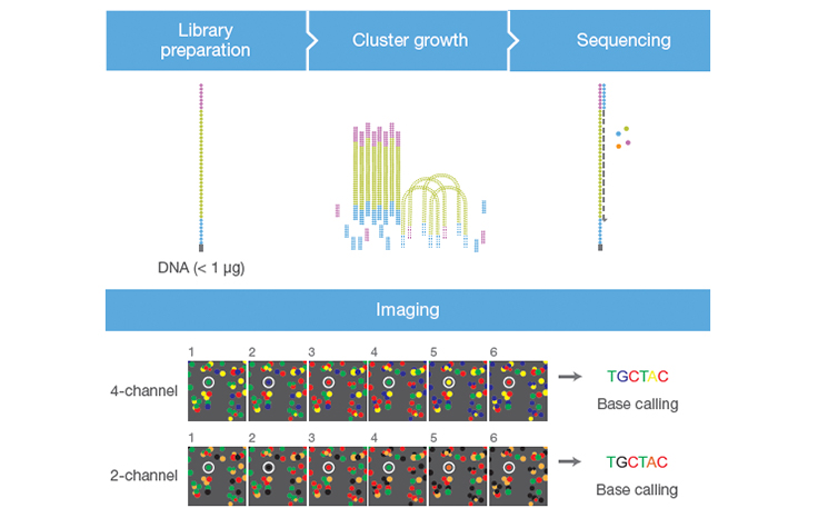
Image Source: Illumina Website

Check out this short, 5 minute video for a quick primer on Illumina sequencing.

For more than a decade, 4 different dye terminator colors were used (T = green, G = blue, C = Red, A = yellow), just like Sanger sequencing. This is called 4-color sequencing. Illumina realized they could speed up sequencing by eliminating two of the colors altogether, reducing the sequencing time by 50%. This is called two-color sequencing. There are only two colored fluorophores used now:

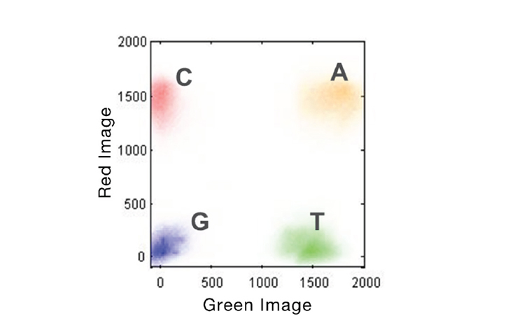
If a base lights up green, it’s a T. If a base lights up red, it’s a C. If a base lights up yellow, it’s A — meaning they mixed red and green fluorphores together for the “A” cycle. If it’s G, there’s no fluorophore, meaning it’s a dark cycle and no light was emitted. The axis of the figure below show the intensity of each base, measured in green versus red intensity.

Image Source Illumina Website

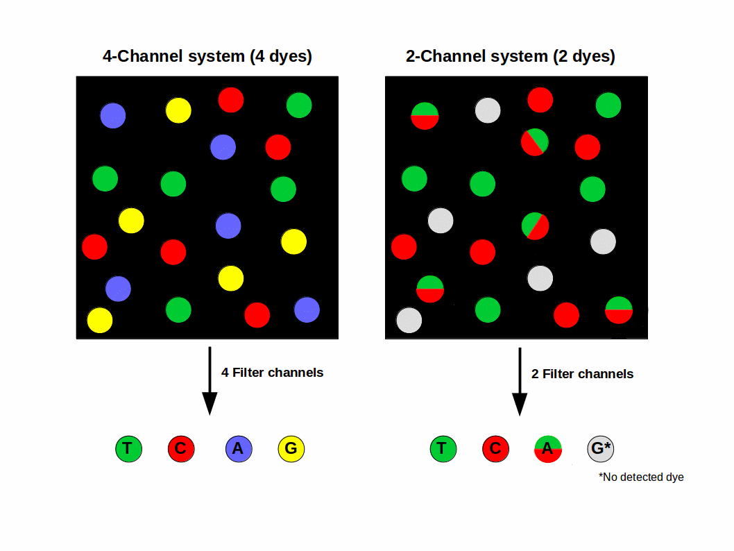
Image Source EC Seq Bioinformatics Website

Do you have two colors or four colors in Illumina?

Step 2: Learn how quality scores in Illumina work

No sequencing technology is perfect (yet), and errors occur at some frequency. It’s important to understand the source of these kinds of errors, because 1) they impact the downstream analyses you want to do, and 2) so you can account for them. Illumina has the lowest per-base error rate of any modern sequencing platform, which is why it is often employed for variant calling during resequencing.

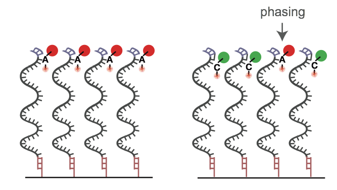
The reasons for errors during the base calling process are diverse. In most cases the emitted light signal of a cluster is disturbed. In this context, it is important to know that the detected light signal is always a sum of single signals from thousands of molecules within one cluster. Typical reasons for a polluted cluster light signal can be phasing (see quality decrease over illumina reads), overlapping clusters and not uniform clusters because of an error in the cluster generation (bridge amplification) step. This can often lead to a gradual degradation of signal over the course of sequencing a molecule. Because the probability of errors fluctuates and differs from cluster to cluster and from cycle to cycle it is necessary and useful to indicate a quality for each called and recorded base expressed in a score.

On the left, a perfect sequencing run with many molecules acting the same within a single cluster. On the right, an example of “phasing”, where the dNTP blocker nucleotide isn’t cleaved, polluting the light signal in the cluster. Image Source EC Seq Bioinformatics Website

In the last few years, especially with the introduction of Illumina’s bigger machines like the NovaSeq6000, the data produced by the machine is becoming unwieldy. One source of data bloating was that every single nucleotide of every single read had a quality score attached to it. The quality score (Q score) with the attached probability of error (P_error) was given a different ASCII code:

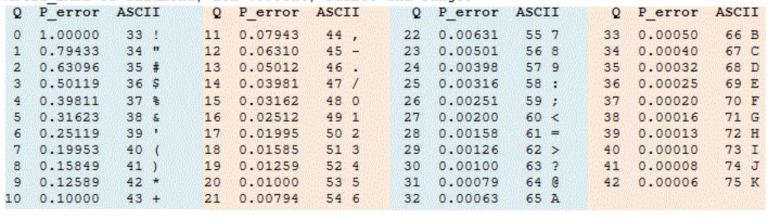
Phred33 offset ASCII table.

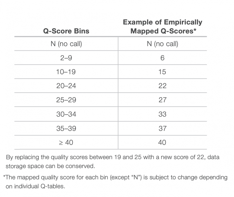
Illumina’s solution to this issue is to not report the quality score of every single nucleotide. Instead, quality scores are binned into 4 or 8 categories of qualities. See the table below for an example of how quality scores can be binned into 8 Q-score categories. In the example below, if a base has a quality score of 7, it gets changed to a “6”. This saves space because when compression algorithms or formats (like gzip, bzip, .bam) compress data, repeated stretches of the same byte (like a quality score bin value) can be very efficiently compressed, resulting in smaller file sizes. In practice, it hasn’t really mattered much to us; binning actually saves us computational time when we trim the data and very few people really needed to know the Q score of every single base.

Task B

Many programs have been written to “clean” Illumina sequencing data. Some common examples are trimmomatic, TrimGalore!, and my personal favorite, Fastp. Fastp is exceptionally fast, and the defaults are excellent. It will automatically trim your fastq dataset with reasonable defaults, including automatically identifying and trimming the adapter sequences that might be present in your data.

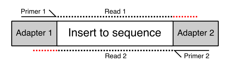
The structure of an Illumina-ready molecule for sequencing is below. The “insert” is your biological sequence (e.g. a piece of DNA or RNA), flanked on both sides by “adapter” sequence that is required for binding to the flow cell. The first read (R1) initiates sequencing at Primer 1, and reads through the insert sequence on the top strand. Depending on the length of the insert, and the chosen sequencing read length, sometimes you can sequencing into the adapter on the other side of the molecule (shown by the red dots). These adapter sequences at the 3′ ends of reads need to be removed. They are not true biological sequence!

Image Source: QCFail.com Website

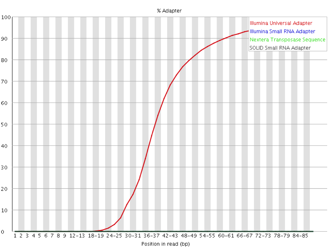
QC Fail Sequencing » Read-through adapters can appear at the ends of sequencing reads These issues are visible in the fastqc plots, like the example below, which shows the Illumina Universal Adapter being present in a high frequency of molecules starting ~35 nucleotides. The insert must be very short here:

Image Source: QCFail.com Website

Similarly, remember how chemistry issues like “phasing” can lead to signal degradation over time? Quality scores often start to drop as the sequencing moves towards the 3′ end of each molecule. This is normal, and we can detect this in fastqc plots. Below is an example:

Image Source EC Seq Bioinformatics Website

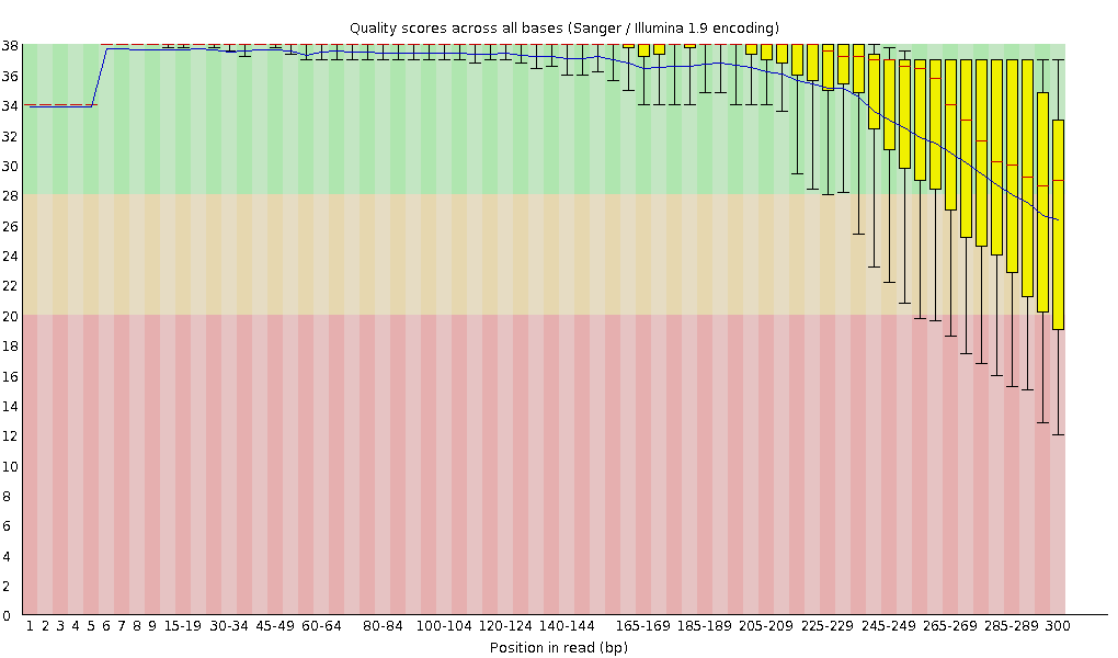
• Why does the per base sequence quality decrease over the read in Illumina?

• Does the Toomer’s Oak data display this trend? Let’s look at the fastqc plots you made.

Install fastp

Read the github page, and install fastp using Conda. Make sure you’re in your “toomers” environment (or whatever you decided to name it).

There are many ways to run fastp to output cleaned reads. You can 1) stream the reads directly to the standard out, so that you can pipe them into another program (e.g. a read aligner like BWA or bowtie), 2) write the cleaned reads to a separate file (which takes up space), or 3) output nothing except for the cleaned read statistics. For this lab, we’ll do #3. In the very near future future, since fastp is so quick to run, we will use the “streaming” option #1, and make use of pipes. This saves us a lot of storage — do we need to keep a copy of the raw data, plus a copy of the cleaned data? Not really*

Note

There are caveats here we will talk about in lab.

Use the same raw Illumina whole genome shotgun data that you used in the last lab. read1 is the file that ends in R1, and read2 is the file that ends in R2. Insert the correct path to the reads, either the raw data from /scratch or your softlinked files in your own directory. The simplest way to run fastp to only generate a quality report of our data is:

fastp -i read1 -I read2
# yeah, it's that easy.

Use the ampersand (&) to start this job in the background. Ask google or your classmates if you can’t remember how. This job will take a few hours.

After the run has finished, run MultiQC in the ~/toomers-genome/ directory to aggregate your fastqc and fastp results.

Mastering Content

What depth of coverage did I sequence to?

A question we often ask — “Did I sequence deeply enough?”.

Next-generation shotgun sequencing approaches require sequencing every base in a sample several times for two reasons:

• You need multiple observations per base to come to a reliable base call.

• Reads are not distributed evenly over an entire genome, simply because the reads will sample the genome in a random and independent manner. Therefore many bases will be covered by fewer reads than the average coverage, while other bases will be covered by more reads than average. You need to account for this in your planning.

This is expressed by the coverage metric, which is the number of times a genome has been sequenced (the depth of sequencing). For applications where you aim to sequence only a defined subset of an entire genome, like targeted resequencing or RNA sequencing, coverage means the amount of times you sequence that subset. For example, for targeted resequencing, coverage means the number of times the targeted subset of the genome is sequenced. In this case, we want to know the sequencing coverage of the whole genome; in other words, how many times did we sequence each nucleotide of the oak tree, on average?

The general equation for computing coverage is: - C = LN / G - C stands for coverage - G is the haploid genome length - L is the read length - N is the number of reads

Assume that the diploid genome size of our Toomers Oak is 1.5 Gigabases. What coverage of Illumina read depth did we sequence to?